Modeling distributions on Riemannian manifolds is a crucial component in understanding non-Euclidean data that arises, e.g., in physics and geology. We propose a class of flows that uses convex potentials from Riemannian optimal transport. These are universal and can model distributions on any compact Riemannian manifold without needing domain knowledge of the manifold to be integrated into the architecture. We demonstrate that these flows can model standard distributions on spheres, and tori, on synthetic and geological data.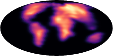
Riemannian Optimal Transport
Optimal transportation provides the foundational toolbox for our studies of transporting distributions. The Monge problem shown below is widely-studied and finds an optimal transport (OT) map t that pushes the distribution $\mu$ forward to $\nu$ at a minimum cost.
$$
\min_{t\in U(\mu,\nu)}\int_\mathcal{M} c(x,t(x))d\mu.
$$ where $U(\mu,\nu)$ is the set of maps such that $t$ transports $\mu$ to $\nu$.
According to McCann’s theorem, the OT is $\exp(-\nabla \phi)$, where $\phi$ is $c$-concave.
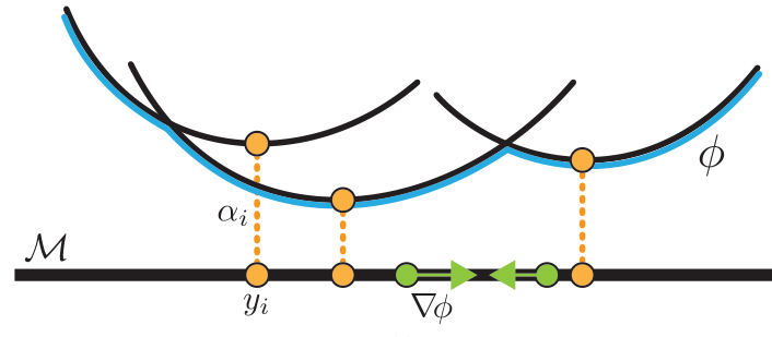
We propose parameterizing $c$-concave potentials as
$$
\phi(x) = \min_{i \in[n]} c(x,y_i)+ \alpha_i,
$$ where $(y_i, \alpha_i)_i$ are learnable parameters.
Theory
A significant part of our paper is on theoretically understanding this class of semidiscrete c-concave functions. We provide two theorems showing that $i)$ our $c$-concave parameterization is universal, and that $ii)$ the transport maps built using them are universal (can push any measure from source to target).
Theorem 1: For compact, boundaryless, smooth manifolds, $(f \vert f(x) = \min_{i \in [n]} c(x,y_i)+ \alpha_i)$ is dense in $(f\vert f \ \text{is c-concave})$
Theorem 2: If $\mu, \nu$ are regular, there exists a sequence of discrete c-concave potentials $\phi_\epsilon$ such that $\exp[-\nabla \phi_\epsilon] \xrightarrow[]{p} t$ where $t$ is the OT map.
Practice
- For expressivity and learnability, we consider a deep composition of transformations of the form
$$
s_j(x) = \exp[-\nabla_x \phi_j(x)], \ \ \ \ j=1,\ldots, T.
$$
In order for to apply gradient-based methods for learning our model parameters, we smooth the discrete c-concave layers, replacing the $\min$ by a smooth $\min$
$$
\min_\gamma(a_1,\ldots, a_n) = -\gamma \log \sum_{i=1}^n \exp{-\frac{a_i}{\gamma}}
$$We train our transport maps leveraging normalizing flow techniques, and consider standard density estimation losses (NLL, KL).
Applications
We showcase a number of applications of our RCPMs, on both spheres and tori, for synthetic and real data.
Sphere, synthetic data: We first consider common synthetic benchmarks to evaluate compare our models to previous methods on the sphere.
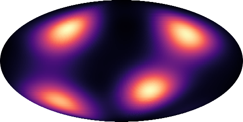
Figure 3: RCPM trained on a four-modal benchmark on the sphere. Torus, synthetic data: We also consider a synthetic example on the torus, in order to demonstrate the generality of our approach.
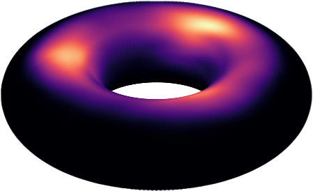
Figure 4: We trained a 6-block RCPM in the density estimation setting. The base distribution is the uniform distribution on the sphere and the target $\nu$ is the ground of current earth.. Sphere, geological data: We then go on to show a case study using land masses from historical Earth to modern Earth on the sphere.
Figure 5: Illustration of a flow induced by a Riemannian Convex Potential Map (RCPM) trained on earth data living on the sphere.
Our model also allows to obtain geodesics between samples from the source $\mu$ and the target $\nu$. These geodesics contain information about how the mass could have moved across time.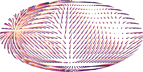
Figure 6: Plot of the transport geodesics arising from a 1-block RCPM trained with source being old earth and target being current earth. We observe that samples stretch according to continental movements.