Actually Sparse Variational Gaussian Processes

Gaussian processes infamously suffer from an $\mathcal{O}(N^3)$ computational complexity and $\mathcal{O}(N^2)$ memory requirements, rendering them intractable for even medium sized datasets where $N\gtrsim 10,000$. Sparse variational Gaussian processes have been developed to alleviate some of the pains of scaling GPs to large datasets by approximating the exact GP posterior with a variational distirbution conditioned on a small set of inducing variables designed to summarise the dataset. However, even sparse GPs can become computationally expensive, limited by the number of inducing points one can use which is particularly troublesome when modelling long timeseries, or fast varying spatial data with very low lengthscales.

In our recent paper at AISTATS 2023, we propose Actually sparse variational Gaussian processes (AS-VGP), a sparse inter-domain inducing approximation that relies on sparse linear algebra to drastically speed up matrix operations and reduce memory requiremnts during inference and training. This enables us to very efficiently use tens of thousands of inducing variables, where other approaches have previsouly failed.

Sparse Variational Gaussian Processes

Sparse Variational Gaussian proesses¹ (SVGPs) leverage inducing points and variational inference to construct a low-rank approximation to the true GP posterior, $$q(f)=\int p(f|\mathbf{u}) q(\mathbf{u}) d\mathbf{u} = \mathcal{N}(\mu, \Sigma)$$

$$\mathbf{u}= \{ f(\mathbf{z}_m) \} _{m=1} ^M $$

For a Gaussian likelihood, the moments of the optimal variational distribution can be computed exactly and we can optimise the kernel hyperparameters by maximisng the ELBO,

$$ \mathcal{L}_{ELBO} = \log \mathcal{N}(\mathbf{y} | \mathbf{0}, \mathbf{K _{fu}} \mathbf{K} _{\mathbf{uu}} ^{-1}\mathbf{K _{uf}}+\sigma ^2 _n\mathbf{I}) - \frac{1}{2}\sigma _n ^{-2} \text{tr}(\mathbf{K _{ff}}-\mathbf{K _{fu}}\mathbf{K} _{\mathbf{uu}} ^{-1}\mathbf{K _{uf}}) $$

where $\mathbf{K_{uu}}=[k(z_i, z_j)]^M_{i,j=1}$ and $\mathbf{K_{uf}}=[k(z_m, x_n)]^{M,N}_{m,n=1}$

Computing the ELBO requires 3 distinct matrix operations:

1. Dense matrix multiplication $\mathbf{K_{uf}}\mathbf{K_{fu}}$ at a cost of $\mathcal{O}(NM^2)$
2. Dense Cholesky factorisation of $\mathbf{K_{uu}}$ at a cost of $\mathcal{O}(M^3)$
3. Dense Cholesky factorisation of $(\mathbf{K_{uu}} + \sigma^{-2}\mathbf{K_{uf}}\mathbf{K_{fu}})$ at a cost of $\mathcal{O}(M^3)$

Inter-Domain Variational Gaussian Processes

Inter-domain GPs^{2 3} generalise the idea of inducing variables by instead conditioning the variational distribution on a linear transformation $\mathcal{L}_{m} $ of the GP,

$$ u_{m}= \mathcal{L}_{m} f(\cdot) = \int g(\cdot,z_m)f(z _m) dz _m $$

Variational Fourier features (VFF)⁴ is an inter-domain variational GP approximation that constructs inducing features as a Matern RKHS projection of the Gaussian process onto a set of Fourier basis functions, $$u_m=\langle f, \phi_m\rangle_{\mathcal{H}}$$ where $\langle \cdot, \cdot \rangle_\mathcal{H}$ denotes the Matern RKHS inner product, and $\phi_0(x)=1, \phi_{2i-1}(x) = \cos(\omega_i x), \phi_{2i}=\sin(\omega_i x)$ are the Fourier basis functions. This results in the following covariance matrices,

$$\mathbf{K_{uu}}=[\langle\phi_i, \phi_j\rangle_\mathcal{H}]^M_{i,j=1},\qquad \mathbf{K_{uf}}=[\phi_m(x_n)]^{M,N}_{m,n=1},$$

where due to the reproducing property, the cross-covariance matrix $\mathbf{K_{uf}}$ is equivalent to evaluating the Fourier basis and is is indepent of of kernel hyperparameters and $\mathbf{K_{uu}}$ is a block-diagonal matrix.

The additional matrix structures induced by VFF reduce computing the ELBO to the following 3 matrix operations:

1. One-time dense matrix multiplication $\mathbf{K_{uf}}\mathbf{K_{fu}}$ at a cost of $\mathcal{O}(NM^2)$
2. Block-diagonal Cholesky factorisation of $\mathbf{K_{uu}}$ at a cost of $\mathcal{O}(M)$
3. Dense Cholesky factorisation of $(\mathbf{K_{uu}} + \sigma^{-2}\mathbf{K_{uf}}\mathbf{K_{fu}})$ at a cost of $\mathcal{O}(M^3)$

Although an improvement upon SVGP, $\mathbf{K_{uf}}$ is still a dense matrix and therefore in VFF we are still required to compute a dense Cholesky factor of the $M\times M$ matrix $\mathbf{K_{uu}} + \sigma^{-2} \mathbf{K_{uf}}\mathbf{K_{fu}}$ which costs $\mathcal{O}(M^3)$ and limits the number of inducing points one can use.

B-Spline Inducing Features

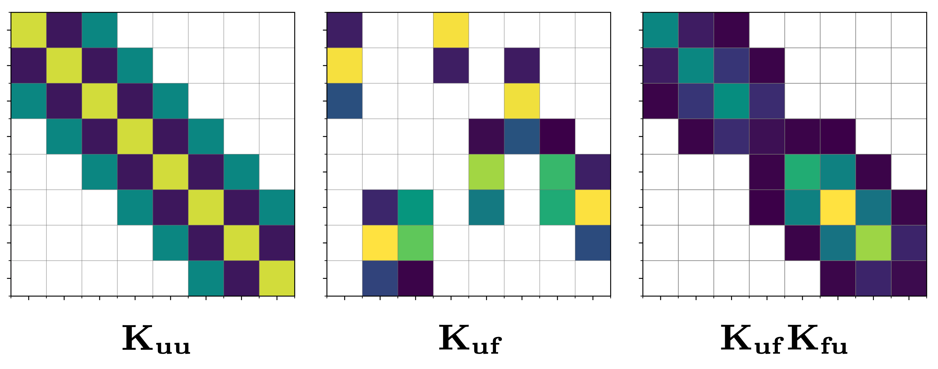
To overcome these issues and scale SVGPs to tens of thousands of inducing points, we introduce B-spline inducing features. The core idea is to use the same RKHS projections as in VFF, except to project the GP onto a set of compactly supported B-spline basis functions. Unlike in VFF, the inducing features are localised by the nature of their compact support, such that $\mathbf{K_{uu}}$, $\mathbf{K_{uf}}$ and the matrix product $\mathbf{K_{uf}}\mathbf{K_{fu}}$ are all sparse matrices. See figure x.

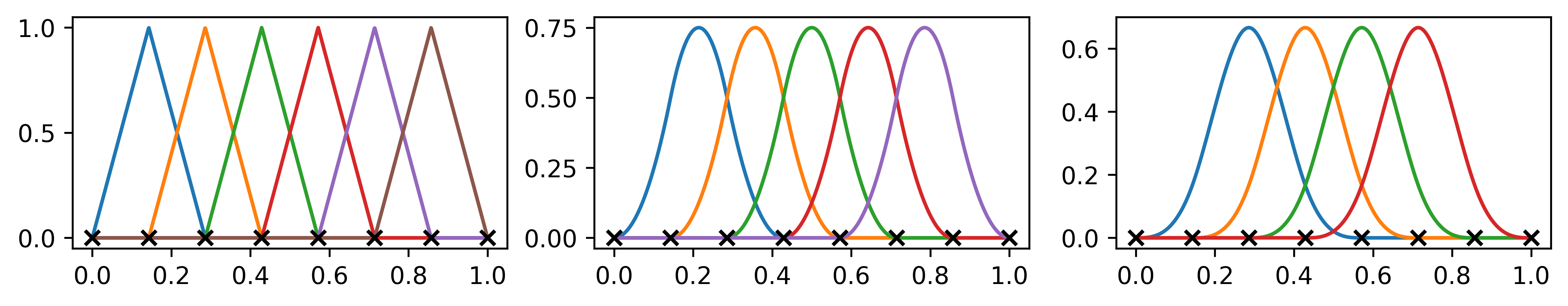
Fig 2. (left) 1st-order B-spline basis (middle) 2nd-order B-spline basis (right) 3rd-order B-spline basis

Consequently computing the ELBO is now reduced to only working with sparse matrices, and using the banded operators package can be computed without ever having to instantiate a dense matrix,

1. One-time sparse matrix multiplication $\mathbf{K_{uf}}\mathbf{K_{fu}}$ at a cost of $\mathcal{O}(N)$
2. Band-diagonal Cholesky factorisation of $\mathbf{K_{uu}}$ at a cost of $\mathcal{O}(M(k+1)^2)$
3. Band-diagonal Cholesky factorisation of $(\mathbf{K_{uu}} + \sigma^{-2}\mathbf{K_{uf}}\mathbf{K_{fu}})$ at a cost of $\mathcal{O}(M(k+1)^2)$

Training AS-VGP therefore requires a one-off precomputation cost linear in the number of data points followed by optimisation of the ELBO which scales linearly in the number of inducing-points. This allows us to scale SVGP to both millions of data-points and tens of thousands of inducing points.

Fig 3. Illustration of the linear scaling in computation of the ELBO and independence on computing the product $\mathbf{K_{uf}K_{fu}}$ w.r.t. the number of inducing points.

Summary

In conlcusion, we present AS-VGP a novel sparse variational inter-domain GP model wherein the inducing features are defined as RKHS projections of the GP onto a set of compactly-supported B-spline basis functions. The resulting covariance matrices are sparse allowing us to use sparse linear algebra and scale GPs to tens of thousands of inducing variables. We also highlight how our method works best for low dimensional problems such as time-series and spatial data.

References

Titsias, M., 2009, April. Variational learning of inducing variables in sparse Gaussian processes. In Artificial intelligence and statistics (pp. 567-574). PMLR. ↩︎
Lázaro-Gredilla, M. and Figueiras-Vidal, A., 2009. Inter-domain Gaussian processes for sparse inference using inducing features. Advances in Neural Information Processing Systems, 22. ↩︎
Van der Wilk, M., Dutordoir, V., John, S.T., Artemev, A., Adam, V. and Hensman, J., 2020. A framework for interdomain and multioutput Gaussian processes. arXiv preprint arXiv:2003.01115. ↩︎
Hensman, J., Durrande, N. and Solin, A., 2017. Variational Fourier Features for Gaussian Processes. J. Mach. Learn. Res., 18(1), pp.5537-5588. ↩︎